Assumptions
I’m assuming you’ve downloaded VS Code because everyone uses it or Cursor or some other IDE. If you haven’t, you should. Go through the steps of learning how to open files and all that and come back here. Especially after you learn how to use the terminal, because I’m going to shout stuff out like
run this
mkdir some_directory
cd some_directory
and you need to know what I mean, so quick intro to linux or command line would behoove anyone new to scientific computing. If you’re not using Linux on a laptop/desktop, buy a laptop, a wireless keyboard/mouse combo, and a monitor and start today. You can’t do this shit on a fucking phone or a tablet. Don’t try.
Install uv
Go read how to install uv yourself. Too lazy to do that. Okay here
curl -LsSf https://astral.sh/uv/install.sh | shLet’s create a directory somewhere to run our code
# I always use something like this
mkdir -p ~/src
cd ~/src
# Let's create a directory for our work
mkdir scicomp_py
cd scicomp_py
# Initialize uv
uv init .
uv venv
source .venv/bin/activate
# You should have installed cursor or vs code or something
code . # or cursor .
Okay now you’re ready to rock and roll. Other people might tell you to use conda or even just use pip with your system install. We are not those people. I used to use my system install for years until I got into installing conda at work.
As I understand continuum analytics or whatever the company behind conda decided they were going to get serious about licensing so yeah no time like the present to switch to uv. Conda forge/miniforge whatever is great, but we’re going to use uv.
Install numpy
Okay now let’s get this party started.
# Let's get set up to do numerical computing in python
uv add numpy
# We want
uv add IPython
# Install matplotlib to plot graphs and stuff
uv add matplotlib
# Install jupyterlab to run notebooks
uv add jupyterlab
uv sync
and finally
uv run -m IPythonThis is the IPython REPL, which is going to be your best friend. Can’t get your notebook working? Some stupid kernel problems or VS Code fighting your uv installation? Fuck it, paste it into ipython
This is my debugger. There are many like it, but this one is mine. Python is an interpreted language, so you can always just run it step by step right in the REPL, which is what I want you to do right now.
ENOUGH TALK! LET’S RUN SOME CODE
Alright already damn. Give us a second. I’m assuming people have never run a jupyter notebook or opened a terminal in their life sheesh.
Again you can download this notebook by clicking the download button above and copy it to
~/src/scicomp_py/chapter-01.ipynbAgain you can download this notebook by clicking the download button above and copy it to
~/src/scicomp_py/chapter-01.ipynbor you can create a new file through IDE GUI, call it chapter-01.ipynb, and open it in your IDE.
or you can do the following in a terminal
touch chapter-01.ipynband THEN open that file in your IDE.
And if all else fails, use the IPython REPL. Copy/paste this in there line by line. It works.
OKAY RUN THIS
import numpy as np
# Okay this is a "hello world" of numerical computing.
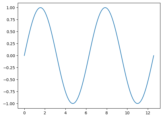
# We're going to make a cosine wave.
x = np.linspace(0,4*np.pi, 100)
y = np.sin(x)
Okay let’s take a look at x
print(x)[ 0. 0.12693304 0.25386607 0.38079911 0.50773215 0.63466518
0.76159822 0.88853126 1.01546429 1.14239733 1.26933037 1.3962634
1.52319644 1.65012947 1.77706251 1.90399555 2.03092858 2.15786162
2.28479466 2.41172769 2.53866073 2.66559377 2.7925268 2.91945984
3.04639288 3.17332591 3.30025895 3.42719199 3.55412502 3.68105806
3.8079911 3.93492413 4.06185717 4.1887902 4.31572324 4.44265628
4.56958931 4.69652235 4.82345539 4.95038842 5.07732146 5.2042545
5.33118753 5.45812057 5.58505361 5.71198664 5.83891968 5.96585272
6.09278575 6.21971879 6.34665183 6.47358486 6.6005179 6.72745093
6.85438397 6.98131701 7.10825004 7.23518308 7.36211612 7.48904915
7.61598219 7.74291523 7.86984826 7.9967813 8.12371434 8.25064737
8.37758041 8.50451345 8.63144648 8.75837952 8.88531256 9.01224559
9.13917863 9.26611167 9.3930447 9.51997774 9.64691077 9.77384381
9.90077685 10.02770988 10.15464292 10.28157596 10.40850899 10.53544203
10.66237507 10.7893081 10.91624114 11.04317418 11.17010721 11.29704025
11.42397329 11.55090632 11.67783936 11.8047724 11.93170543 12.05863847
12.1855715 12.31250454 12.43943758 12.56637061]
Now let’s take a look at y
print(y)[ 0.00000000e+00 1.26592454e-01 2.51147987e-01 3.71662456e-01
4.86196736e-01 5.92907929e-01 6.90079011e-01 7.76146464e-01
8.49725430e-01 9.09631995e-01 9.54902241e-01 9.84807753e-01
9.98867339e-01 9.96854776e-01 9.78802446e-01 9.45000819e-01
8.95993774e-01 8.32569855e-01 7.55749574e-01 6.66769001e-01
5.67059864e-01 4.58226522e-01 3.42020143e-01 2.20310533e-01
9.50560433e-02 -3.17279335e-02 -1.58001396e-01 -2.81732557e-01
-4.00930535e-01 -5.13677392e-01 -6.18158986e-01 -7.12694171e-01
-7.95761841e-01 -8.66025404e-01 -9.22354294e-01 -9.63842159e-01
-9.89821442e-01 -9.99874128e-01 -9.93838464e-01 -9.71811568e-01
-9.34147860e-01 -8.81453363e-01 -8.14575952e-01 -7.34591709e-01
-6.42787610e-01 -5.40640817e-01 -4.29794912e-01 -3.12033446e-01
-1.89251244e-01 -6.34239197e-02 6.34239197e-02 1.89251244e-01
3.12033446e-01 4.29794912e-01 5.40640817e-01 6.42787610e-01
7.34591709e-01 8.14575952e-01 8.81453363e-01 9.34147860e-01
9.71811568e-01 9.93838464e-01 9.99874128e-01 9.89821442e-01
9.63842159e-01 9.22354294e-01 8.66025404e-01 7.95761841e-01
7.12694171e-01 6.18158986e-01 5.13677392e-01 4.00930535e-01
2.81732557e-01 1.58001396e-01 3.17279335e-02 -9.50560433e-02
-2.20310533e-01 -3.42020143e-01 -4.58226522e-01 -5.67059864e-01
-6.66769001e-01 -7.55749574e-01 -8.32569855e-01 -8.95993774e-01
-9.45000819e-01 -9.78802446e-01 -9.96854776e-01 -9.98867339e-01
-9.84807753e-01 -9.54902241e-01 -9.09631995e-01 -8.49725430e-01
-7.76146464e-01 -6.90079011e-01 -5.92907929e-01 -4.86196736e-01
-3.71662456e-01 -2.51147987e-01 -1.26592454e-01 -4.89858720e-16]
There’s a better way to visualize data in python of course. There are a hundred different packages out there now, from bokeh to ggplot, but we’re going to start with the tried and true matplotlib.
# Let's plot our function
import matplotlib.pyplot as plt
plt.plot(x, y)
plt.show()
So seems like no big deal eh?
Wrong!
We’ve managed to connect our mathematical entities
with code we can run
import numpy as np
x = np.linspace(0,4*np.pi, 100)
y = np.sin(x)
The most useful function in Python
I’m talking about dir() of course!
The second most helpful is help(). Let’s start by using the second to tell us about the first!
help(dir)Help on built-in function dir in module builtins:
dir(...)
Show attributes of an object.
If called without an argument, return the names in the current scope.
Else, return an alphabetized list of names comprising (some of) the attributes
of the given object, and of attributes reachable from it.
If the object supplies a method named __dir__, it will be used; otherwise
the default dir() logic is used and returns:
for a module object: the module's attributes.
for a class object: its attributes, and recursively the attributes
of its bases.
for any other object: its attributes, its class's attributes, and
recursively the attributes of its class's base classes.
items_in_numpy = [x for x in dir(np) if not x.startswith('_')]

for item in items_in_numpy[:10]:
    print(item)
False_
ScalarType
True_
abs
absolute
acos
acosh
add
all
allclose
for item in items_in_numpy[-10:]:
    print(item)
vdot
vecdot
vecmat
vectorize
void
vsplit
vstack
where
zeros
zeros_like
help(np.zeros_like)Help on _ArrayFunctionDispatcher in module numpy:
zeros_like(a, dtype=None, order='K', subok=True, shape=None, *, device=None)
Return an array of zeros with the same shape and type as a given array.
Parameters
----------
a : array_like
The shape and data-type of `a` define these same attributes of
the returned array.
dtype : data-type, optional
Overrides the data type of the result.
order : {'C', 'F', 'A', or 'K'}, optional
Overrides the memory layout of the result. 'C' means C-order,
'F' means F-order, 'A' means 'F' if `a` is Fortran contiguous,
'C' otherwise. 'K' means match the layout of `a` as closely
as possible.
subok : bool, optional.
If True, then the newly created array will use the sub-class
type of `a`, otherwise it will be a base-class array. Defaults
to True.
shape : int or sequence of ints, optional.
Overrides the shape of the result. If order='K' and the number of
dimensions is unchanged, will try to keep order, otherwise,
order='C' is implied.
device : str, optional
The device on which to place the created array. Default: None.
For Array-API interoperability only, so must be ``"cpu"`` if passed.
.. versionadded:: 2.0.0
Returns
-------
out : ndarray
Array of zeros with the same shape and type as `a`.
See Also
--------
empty_like : Return an empty array with shape and type of input.
ones_like : Return an array of ones with shape and type of input.
full_like : Return a new array with shape of input filled with value.
zeros : Return a new array setting values to zero.
Examples
--------
>>> import numpy as np
>>> x = np.arange(6)
>>> x = x.reshape((2, 3))
>>> x
array([[0, 1, 2],
[3, 4, 5]])
>>> np.zeros_like(x)
array([[0, 0, 0],
[0, 0, 0]])
>>> y = np.arange(3, dtype=float)
>>> y
array([0., 1., 2.])
>>> np.zeros_like(y)
array([0., 0., 0.])
help(np.array)Help on built-in function array in module numpy:
array(...)
array(object, dtype=None, *, copy=True, order='K', subok=False, ndmin=0,
like=None)
Create an array.
Parameters
----------
object : array_like
An array, any object exposing the array interface, an object whose
``__array__`` method returns an array, or any (nested) sequence.
If object is a scalar, a 0-dimensional array containing object is
returned.
dtype : data-type, optional
The desired data-type for the array. If not given, NumPy will try to use
a default ``dtype`` that can represent the values (by applying promotion
rules when necessary.)
copy : bool, optional
If ``True`` (default), then the array data is copied. If ``None``,
a copy will only be made if ``__array__`` returns a copy, if obj is
a nested sequence, or if a copy is needed to satisfy any of the other
requirements (``dtype``, ``order``, etc.). Note that any copy of
the data is shallow, i.e., for arrays with object dtype, the new
array will point to the same objects. See Examples for `ndarray.copy`.
For ``False`` it raises a ``ValueError`` if a copy cannot be avoided.
Default: ``True``.
order : {'K', 'A', 'C', 'F'}, optional
Specify the memory layout of the array. If object is not an array, the
newly created array will be in C order (row major) unless 'F' is
specified, in which case it will be in Fortran order (column major).
If object is an array the following holds.
===== ========= ===================================================
order no copy copy=True
===== ========= ===================================================
'K' unchanged F & C order preserved, otherwise most similar order
'A' unchanged F order if input is F and not C, otherwise C order
'C' C order C order
'F' F order F order
===== ========= ===================================================
When ``copy=None`` and a copy is made for other reasons, the result is
the same as if ``copy=True``, with some exceptions for 'A', see the
Notes section. The default order is 'K'.
subok : bool, optional
If True, then sub-classes will be passed-through, otherwise
the returned array will be forced to be a base-class array (default).
ndmin : int, optional
Specifies the minimum number of dimensions that the resulting
array should have. Ones will be prepended to the shape as
needed to meet this requirement.
like : array_like, optional
Reference object to allow the creation of arrays which are not
NumPy arrays. If an array-like passed in as ``like`` supports
the ``__array_function__`` protocol, the result will be defined
by it. In this case, it ensures the creation of an array object
compatible with that passed in via this argument.
.. versionadded:: 1.20.0
Returns
-------
out : ndarray
An array object satisfying the specified requirements.
See Also
--------
empty_like : Return an empty array with shape and type of input.
ones_like : Return an array of ones with shape and type of input.
zeros_like : Return an array of zeros with shape and type of input.
full_like : Return a new array with shape of input filled with value.
empty : Return a new uninitialized array.
ones : Return a new array setting values to one.
zeros : Return a new array setting values to zero.
full : Return a new array of given shape filled with value.
copy: Return an array copy of the given object.
Notes
-----
When order is 'A' and ``object`` is an array in neither 'C' nor 'F' order,
and a copy is forced by a change in dtype, then the order of the result is
not necessarily 'C' as expected. This is likely a bug.
Examples
--------
>>> import numpy as np
>>> np.array([1, 2, 3])
array([1, 2, 3])
Upcasting:
>>> np.array([1, 2, 3.0])
array([ 1., 2., 3.])
More than one dimension:
>>> np.array([[1, 2], [3, 4]])
array([[1, 2],
[3, 4]])
Minimum dimensions 2:
>>> np.array([1, 2, 3], ndmin=2)
array([[1, 2, 3]])
Type provided:
>>> np.array([1, 2, 3], dtype=complex)
array([ 1.+0.j, 2.+0.j, 3.+0.j])
Data-type consisting of more than one element:
>>> x = np.array([(1,2),(3,4)],dtype=[('a','<i4'),('b','<i4')])
>>> x['a']
array([1, 3], dtype=int32)
Creating an array from sub-classes:
>>> np.array(np.asmatrix('1 2; 3 4'))
array([[1, 2],
[3, 4]])
>>> np.array(np.asmatrix('1 2; 3 4'), subok=True)
matrix([[1, 2],
[3, 4]])
Keys to the Kingdom
Now we know how to use both np.array and np.zeros_like because of dir() and help().
a = np.array([1, 2, 3])
b = np.zeros_like(a)
print(a)
[1 2 3]
print(b)[0 0 0]
Teach a man to fish...
There are a million and one resources out there that show all of the amazing and wonderful uses of linear algebra and arrays on a computer. No doubt you use some of them almost if not every day. And we’re going to link to those, later.
For right now though, we’re going to call it a day. You’ve made some huge leaps even if it doesn’t feel like it right now. If you’re like “wtf I know this already!?” then good for you. Here’s a cookie 🍪.